

Profiling is the practice of executing code whilst collecting granular metrics; in particular, performance profilers collect information to help reveal where time is being spent in the code during execution. The information collected ranges from the time spent executing each function or line of code to low-level hardware metrics such as achieved memory bandwidth.
Regardless of experience, whether a self-taught or trained programmer, it’s always possible to introduce small inefficiencies into your code that significantly impact performance. These may not impact the correctness of your results, so it’s easy for them to go overlooked. Profiling narrows the scope for optimisation from the entire codebase to potentially just a handful of lines, enabling quick identification of issues that might otherwise be overlooked.
Profile code once it is functionally complete and before release, since performance hotspots often shift as a program evolves. Choose a specific, realistic workflow to profile, because only executed code is measured. For configurable programs, use a shorter but representative setup to reduce time spent profiling while still exercising important code paths. For iterative programs like simulations, profiling a representative subset of iterations is usually enough, as long as it captures the program’s main behaviours.
Most profilers can be used without making changes to your project, however compiled languages such as C/C++, will typically require the build to be configured explicitly for profiling. Some advanced profiling tools can be controlled directly from your code, enabling you to profile a small subset of an otherwise long run.
It’s recommended that most people start profiling with hot-path (otherwise known as hotspot) profiling, which measures how much time is spent executing each function and/or line of code and highlights the most computationally expensive functions and lines. Other styles of profiler exist, such as timeline profilers which are useful for visualising parallel executions, and hardware metric profilers which present low-level hardware performance data for advanced users.
Interpreting Profiling Results
Hot-path profilers are the most general, so they make up the vast majority of profilers. It’s necessary to find a profiler which supports your programming language, however beyond that they’re highly interchangeable. Each profiler has a slightly different method of executing code, but they share common methods of presenting results after the profiled code executes to completion.
The following sub-sections, introduce the three most common methods of visualising results among profiling tools.
Flame and Icicle Graphs
Flame graphs and icicle graphs are standard visualisations for aggregated, function-level profiling data. Flame graphs place the root row at the bottom and grow upwards, while icicle graphs place the root row at the top and grow downwards. Aside from orientation, they are interpreted in exactly the same way.
The root row always contains a single full-width cell, representing the entry point of the profiled execution, typically the main function. Above or below it, depending on the orientation, successive rows show cells corresponding to functions called by their parent. The width of each cell represents the aggregated runtime spent in that function, including time spent in its callees.
Child cells occupy some fraction of the width of their parent. Most functions spend time performing work other than calling child functions, such as control flow, arithmetic, or data manipulation. This unused space produces the stepped appearance characteristic of flame (Figure 1) and icicle (Figure 2) graphs, which gives them their names.
These graphs are typically interactive. Selecting a cell redraws the graph with that function as the new root, making it easier to inspect deeper call hierarchies that may otherwise be difficult to see.
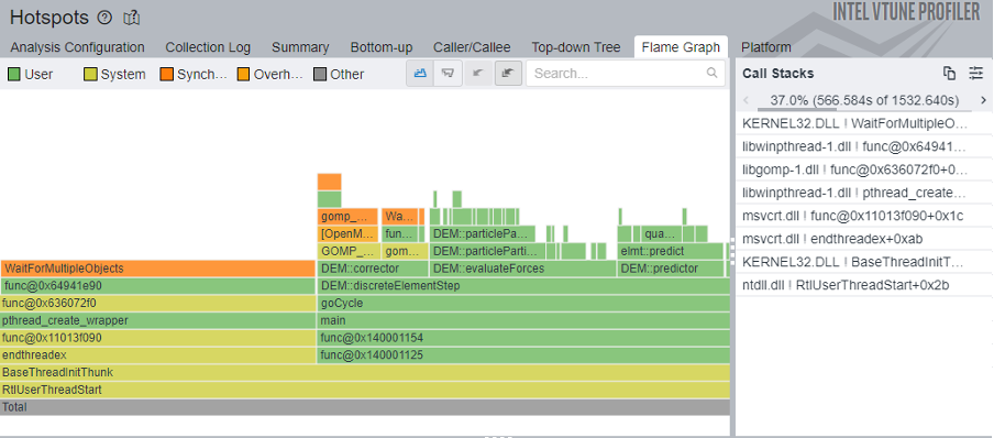
Figure 1. Intel VTune’s hotspots profile Flame Graph tab.
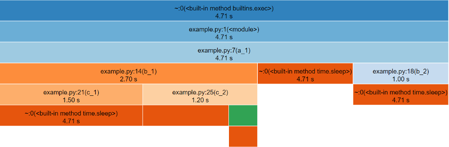
Figure 2. An example of the default ‘icicle’ visualisation provided by snakeviz (visualisation tool for Python’s cProfile).
Table View
Another common way to present function-level profiling data is as a table, often referred to as a profile summary. This lists functions alongside their measured runtime, typically reported both inclusive and exclusive of time spent in child function calls. Some profilers also record how many times each function is invoked, allowing a per-call cost to be derived.
These tables provide a fast way to identify the most computationally expensive functions in a program. However, unlike flame or icicle graphs, they do not naturally convey call hierarchy or the context in which functions are executed.
Depending on the tool, the table may be interactive, allowing rows to be sorted or functions to be selected to jump directly to an annotated source code view (Figure 3). Other profilers provide only a static table representation (Figure 4).
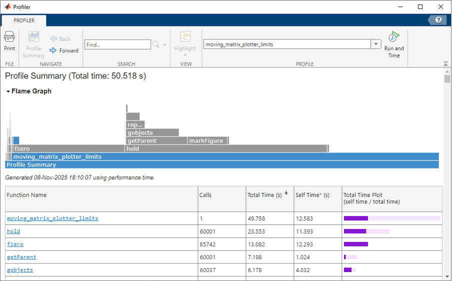
Figure 3. An example of the Profile Summary window showing flame graph top, function table bottom within MATLAB R2025b.
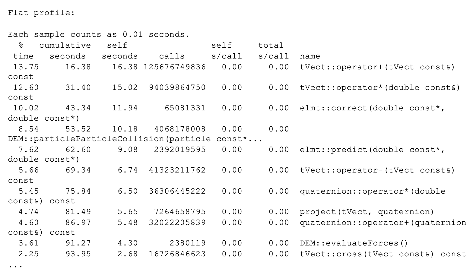
Figure 4. An example of the plain-text Flat profile table output by GProf. (Some function prototypes have been compacted, and inexpensive rows omit)
Inline Code
In contrast to function-level visualisations, line-level profiling results are typically presented inline with the source code. Each line is shown alongside profiling metrics in a pseudo-table layout, often using visual cues such as background shading to indicate relative cost (Figure 5). Lines with high execution time are commonly highlighted with colours, which get darker or warmer corresponding to each line’s expense, making hotspots immediately visible.
This inline representation provides a fast way to identify performance patterns within a function, particularly when scanning large files. It can reveal expensive loops, conditionals, or individual operations that are not obvious from function-level results alone.
For large codebases, which may contain tens or hundreds of thousands of lines, inline views are rarely the primary entry point for analysis. Instead, many profilers require users to navigate from higher-level results, such as function-level summaries, to jump directly to the relevant source locations.
Line-level profiling is most effective once function-level profiling has already narrowed the investigation to a small set of candidate functions. A typical workflow is to begin with function‑level profiling, then drill down to line‑level only where needed. In many cases, function-level results are sufficient on their own, with line-level profiling serving as a deeper diagnostic tool when necessary.
Identifying Optimisations
Once profiling results have been interpreted, the next step is to determine whether there are obvious optimisation opportunities in the components identified as most expensive.
Many of the easiest performance improvements come from eliminating redundant work. This can take several forms. In some cases the issue will be immediately obvious to the code’s author, such as expensive logging, validation, or diagnostics performed on every iteration that could be removed entirely or reduced in frequency. In other cases, profiling highlights expensive calculations, object creation, or other intensive operations that are repeated unnecessarily inside loops and could instead be performed once and reused (for example the profiling report may identify that the majority of the runtime is spent copying).
More subtle forms of redundancy are often hidden behind incorrect library usage. For example, passing an inappropriate data type to a library function, such as a Python list to a NumPy function, may trigger an implicit and expensive conversion on every call.
These issues are frequently logical errors rather than complex performance problems, and they can occur within a few lines of code or across several layers of abstraction.
Other quick optimisations require more experience to recognise. A common example is using a linear search over a collection such as an array to test for membership. While this approach is intuitive, using a set data structure is often far more appropriate and can be orders of magnitude faster for large inputs.
It is difficult to provide a comprehensive checklist for identifying all possible optimisations. If the most expensive components appear reasonable and no obvious issues stand out, it may be that the code is already performing as well as expected. If doubts remain, there are several practical next steps:
- Look for relevant patterns in books or websites related to the language or library you are using.
- Ask a large language model to review a small, self-contained code snippet for performance issues. Providing additional context such as data types and expected input sizes will significantly improve the quality of feedback. Though be aware that LLMs often provide incorrect advice, so you should always verify whether the suggestions actually improve performance and give correct results. Likewise, ensure sharing your code with LLMs complies with your local data-protection policies.
- Request a review from a local Research Software Engineering (RSE) or Research IT team. With profiling results available, experienced developers can often identify potential issues quickly or help investigate less obvious ones.
After applying any optimisation, always re-profile the code and carry out your normal validation. It is important to make sure your optimised code still produces valid results as optimisation changes can introduce subtle correctness issues. A formal test suite is ideal for catching such errors. You may also find at this stage, upon re-profiling, that removing one bottleneck has exposed smaller secondary ones which could be worth optimising too.
Conclusion
A clean profiling report provides additional confidence that your code meets a higher standard of quality, both for running workloads reliably and for publishing reproducible research software. With more experience reviewing your code’s performance, you will find it easier to spot similar issues and potentially even catch them whilst writing code. A profiling report may also help uncover inefficiencies whose removal can reduce overall energy consumption and, in turn, lower the environmental impact associated with running computational workloads.
Now that you’ve read this guide, your next step is to find a profiler you want to use. Perhaps you already have one in mind, if you’re unsure check out some of Reasonable Performance Computing SIG’s profiler mini-guides.
The broad goal of Reasonable Performance Computing SIG is to introduce programmers of all skill levels to the basics of profiling and optimisation. Their website also contains databases of optimisation patterns, and real-world performance case studies. This guide is a concise version of their 4000 word getting started guide.
If you’re instead working with parallel, GPU parallel or even distributed codes you should look into regional and national HPC centres. Many offer training and support for optimising these advanced codes, and ensuring every last ounce of hardware is properly utilised.
Acknowledgements
This guide was written by Robert Chrisholm, and reviewed by Irufan Ahmed.
Contact Robert: